1 Direct LiNGAM Conjecture
In this week and last week, I spent some time digging into the exact non-linear cases for the direct test. More specifically, I visualized the fitting line and points to see how non-linear models work, and the relation between residual and variables to see whether the results fit our assumption.
After digging into the tests, I believe it is time to rethink on the conjecture and give a better illustration.
1.1 Basic Assumption
The basic assumption for Direct LiNGAM Conjecture is that it makes causal direction equivalent with the formula y = f(x) + e(), where f() can be any functions, and e() is a noise with mean 0 (if the mean is not 0, we can put the mean into f() and still get a mean 0 noise). In this case, if we detect a structure like this formula, then we will assume that y is caused by x.
We could notice that if the real causal effect does not satisfy our assumption, then the direct test could be totally wrong. For example, if the noise is relevant with x, or the noise is inside of the function f(), then we can not determine the causal direction correctly, since it is against our assumption.
1.2 Direct Detection
Now the question becomes how to detect such structure. We can notice that for the forward direction (the real causal direction), if we remove the influence of x from y, then the residual, which is the noise, is independent with x. Then in practice, we could fit y with x using a non-linear machine learning model, then run a independence test on the residual and x. If the residual is independent with x, then we could say that we discover a y = f(x) + e() structure.
Notice that we have a high demand on the non-linear machine learning model here, since we need it to remove all the influence of x on y. If the model can not fit the function f() well, then the residual will be dependent on x. Since there are a lot of choices for non-linear model, the through tests would be needed, which is done previously and viewed in visualization.
We could also think what will happen if the real causal doesn't fit out assumption. If the causal is like y = f(x) + e(x), where the variance of noise e() is dependent on x, then in our test, the noise will be dependent with x, and the correct direction can not be detected. If the causal is like y = f(x+e()), the residual we get will also be dependent on x. For example, if y = (x+e())^2 = x^2 + 2x*e()+e()^2, the residual we get will be 2x*e()+e()^2-E[e()^2], which is dependent on x. What's more, if we examine the backward direction, where x = f^(-1)(y)-e(). Then if the inverse function exists, like in this square case, the algorithm will detect that this backward direction is the correct causal direction.
Another question remained is that what if we run the direct test on the reverse direction if the causal effect satisfies our assumption. In fact it is the reverse case we discussed above, that x = f^(-1)(y-e()). The residual we get for this will be dependent on y (I am not quite sure about whether there exists a non-linear function where the residual will be independent with y, here different non-linear function and different kind of noise will have different results). If the relation is linear, then the noise can not be all from normal distribution, which has been proved previously, otherwise for both directions the independence will be detected.
Although in assumption we can detect such structure easily, in practice it may not be that easy since we don't have infinite dataset, and our non-linear model can not always fit the function well. And for some functions, it is just impossible to fit. Therefore, in practice we will run the direct test on both direction and compare the degree of independence. If the margin between two directions are large enough we will decide that the direction with more degree of independence to be the causal direction.
1.3 Non-linear Function Category
When visualization on the direct test results, it turns out that there are multiple cases of non-linear function, which have different results of the algorithm.
1.3.1 Non-monotonic Function
If the function f() here is non-monotonic, then there will be no inverse function, and the reverse direction will test out highly dependence. As long as we can fit the function well, the results would be correct.
For example, we can visualize on square function, the results would be very clear.
Forward direction fitting line and residual
Backward direction fitting line and residual
1.3.2 Function Cannot Be Fitted
Some functions are just simply can not be fitted by a non-linear machine learning model, and for that causal direction, the residual will be dependent and the causal direct can not be detected.
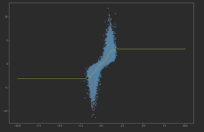
For example, consider function y = 1 / x. If x comes from a noise with mean 0, the function just can not be fitted due to the extreme value.
Forward direction fitting line and residual
1.3.3 Function with 0 derivative in the limit
These functions are like the reverse version of hard-to-fit functions, where the inverse function of them is very hard to fit.
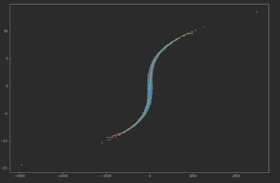
For example, we can consider the function y = tanh(x), where the derivative goes to 0 when x goes to infinite. The forward direction would be easy to detect. The backward direction would result in dependent results, though may not like what we expected that the residuals are dependent, but that we just simply can not fit the model.
Forward direction fitting line and residual
Backward direction fitting line and residual
1.3.4 Function Can Be Fitted
In the end we can examine the cases that the function can be fitted well by the non-linear model for both directions.
We can take y = x^3 as our example. We can observe that the residual in backward direction shows strong dependence on y, as we expected.
Forward direction fitting line and residual
Backward direction fitting line and residual
1.4 Integrating into Because
I rewrite the test_direction function in Probability Module and add self.power into cGraph class to support choice of direction test method. When using power>1, function would use non-linear model to fit, otherwise it would use LiNGAM tanh variant method.
For every test, the non-linear algorithm would run direction test for both directions and calculate the margin. If the margin is large enough, then we could decide that this direction is the correct causal direction. In order to output the results in consistency for both methods, the algorithm would scale the margin, then both methods would use 0.0001 as threshold.
Currently the non-linear method uses KNN (k-nearest neighbor) as non-linear model, and uses at the most 100000 samples to fit.
I also remove the standardize process in the algorithm, since I find that it has just input standardized data at the beginning. After test, it should accelerate about 10% of running time.
2 Plan for Next Week
- Begin working on conditional expectation with machine learning


No comments:
Post a Comment